Bayesian Network
A bayesian network is a probabilistic graphical model where relationship between a set of nodes is represented as a direct acyclic graph. Each node represents a random variable and each edge represents a conditional dependency between the two nodes. Bayesian network has an advantage that it intuitively represents a relationship between variables and provides an efficient way to compute the joint probability distribution.
Consider a following example of a simple bayesian network.
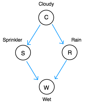
Each node is a binary discrete random variable. The directed arrows show relationships between the variables. Cloudy has an effect on Rain. Weather the grass is wet depends on if the sprinkler is on and if it is raining. The relationship can be causal (like in this example) or non-causal.
From the chain rule, the full joint probability is
Since a node is independent of its non-descendents given its parents, the joint probability can be simplified to
Hidden Variables
A random variable can either be observed or unobserved. A node that represents an unobserved random variable is called a hidden node. If a network is fully observed, then we have the data for all the variables. For our example, a dataset for a fully observed network would look something like this:
| Cloudy | Sprinkler | Rain | Wet |
|---|---|---|---|
| 1 | 0 | 1 | 1 |
| 1 | 0 | 1 | 1 |
| 1 | 0 | 0 | 0 |
| 0 | 1 | 0 | 1 |
| 0 | 1 | 0 | 1 |
| 0 | 0 | 0 | 0 |
The parameters for the conditional probability table of each node can be estimated from the data. From this example data, if we assume each random variable has a binomial distribution and estimate the parameters using the maximun likelihood method, then we get
and so on. For a fully observed network, estimating parameters from data is quite straightforward. However, if one of the nodes is not observed (hidden), then the data might look something like this:
| Cloudy | Sprinkler | Rain | Wet |
|---|---|---|---|
| - | 0 | 1 | 1 |
| - | 0 | 1 | 1 |
| - | 0 | 0 | 0 |
| - | 1 | 0 | 1 |
| - | 1 | 0 | 1 |
| - | 0 | 0 | 0 |
In this case, we don’t have data on Cloudy. If we already have the parameters on this network, then we could do an inference and predict the data on Cloudy. But what if we don’t know the parameters, and we are trying to estimate the parameters from data?
A common approach to estimating model parameters from an incomplete dataset is the expectation-maximization (EM) algorithm. For a full dataset, you can use maximum liklihood to estimate the parameters by finding \( \theta \) that maximizes \( \text{P}(X|\theta) \), where X is the full dataset. With hidden variables, let \( X = X_\text{obs} + X_\text{hidden} \). Instead of maximizing \( \text{P}(X|\theta) \), we find \( \theta \) that maximizes \( \text{P}(X_\text{obs}|\theta) \).
This can be done by first initializing the parameters \( \theta \) to some starting values. Then iterate these two steps until convergence:
- Expectation step: Calculate the expectation of \( \text{P}(X|\theta) \) over \(X_\text{hidden} \) given the current values of \( \theta \).
- Maximization step: Find new values for \( \theta \) that maximize the expectation from step 1.
Each iteration is essentially finding
where \( \theta_i \) is the current value of \( \theta \).
Let’s go through our example. The first step is to initialize the parameters \( \theta \) to some non-uniform values. Let’s say we initialize our network to this:
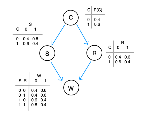
Next is the first iteration of the expectation step. We first calculate \( \text{P}(X_\text{hidden}|X_\text{obs}, \theta_i) \) for each sample in the data. The current \( \theta_i \) has values that we just initialized.
For the first sample, we have
And
Do this for every sample, and we get:
| Cloudy | Sprinkler | Rain | Wet |
|---|---|---|---|
| 0 / 1 | |||
| 0.4/0.6 | 0 | 1 | 1 |
| 0.4/0.6 | 0 | 1 | 1 |
| 0.23/0.77 | 0 | 0 | 0 |
| 0.5/0.5 | 1 | 0 | 1 |
| 0.5/0.5 | 1 | 0 | 1 |
| 0.23/0.77 | 0 | 0 | 0 |
Next is the maximization step. We want to find \( \theta \) that maximizes the above data. Start by finding \( \text{P}(C) \). The maximum likelihood estimation of a binomial parameter is the proportion. So in a regular case, we would count the number of samples with values 1 and divide it by the total number of samples. For our data, we need to multiply the count by the probability \( \text{P}(X_\text{hidden}|X_\text{obs}, \theta_i)\). So we are essentially counting the expected values in the table.
Do this for every random variable: \( \text{P}(S|C), \text{P}(R|C), \text{P}(W|S, R) \) and we get the new conditional probability tables for all the variables. Then iterate each steps until the values of \( \theta \) converge.
bayesnet_em
I wrote a python script to implement the EM algorithm for discrete bayesian networks. The package is available on Github. Bayesnet_em works with Pomegranade to complete dataset with hidden variables by estimating the network parameters and draw samples fromt the distribution to obtain the data for the hidden variables.
Learn more
- Introduction to Bayesian Network
- The Expectation Maximization Algorithm: A Short Tutorial
- Probabilistic Graphical Models: Principles and Techniques, Koller and Friedman, 2009